Lectures 16-17: Continuous random variables

Here are the slides. Reading assignment: BT, Sections 3.1-3.3.

Homework #6

Due, in class: February 22nd

For this homework, you will need to turn in your solutions in two parts. This is for ease of grading by the TAs. Problems 1-3 and 5-6 (+ the extra credit) should be turned in on different sheets of paper (there will be two different piles).

In solving the problem sets, you are allowed to collaborate with fellow students taking the class, but remember that you are required to write up the solutions by yourself or with a single partner. If you do collaborate in any way, you must acknowledge, for each problem, the people you worked with on that problem.

The problems have been carefully chosen for their pedagogical value, and hence might be similar to those given in past offerings of this course at UW, or similar to other courses at other schools.  Using any pre-existing solutions from these sources, for from the web, constitutes a violation of the academic integrity you are expected to exemplify, and is strictly prohibited.

Most of the problems only require one or two key ideas for their solution.  It will help you a lot to spell out these main ideas so that you can get most of the credit for a problem even if you err on the finer details.

A final piece of advice:  Start working on the problem sets early!  Don’t wait until the day (or few days) before they’re due.

Problems

Part one

1. Sandwiches. Suppose you work for a sandwich shop. It costs $10 to buy a vegan sandwich, and you can sell them for $15. Unfortunately, the sandwiches go bad by the end of the day, and you cannot return unsold sandwiches. If your daily demand is a binomial random variable with n=10 and p=1/3, approximately how many vegan sandwiches should you purchase so as to maximize your expected profit?

2. NFLX. Suppose now that you work for Netflix. In a typical hour, there are 50,000 viable users, and each one streams a movie independently with probability p=0.1. You need 10Mb/s of bandwidth to stream a single movie. If your bandwidth is exceeded, you have to drop a stream. Let X = number of movies requested in an hour.
   • Compute E[X]. Using Markov’s inequality, compute the approximate bandwidth you will need so that you drop a stream with probability at most 1/100.

   • Compute Var[X]. Using Chebyshev’s inequality, compute the approximate bandwidth you will need so that you drop a stream with probability at most 1/100.

   • Finally, compute your bandwidth requirement for the same setting using a Chernoff bound.

3. Entropy. A coin with probability p=2/3 of coming up heads is flipped 6 times. Let X = the total number of heads. Compute the entropy of X. Your answer should be in term of bits.

   [Hint: Look in the BT book, or the definition on the wikipedia page.]

Part two

1. You have an array holding 6 numbers, and you run the following algorithm to find the max of those numbers:

   
   max = a[0];
   for(i = 1; i < 6; i++) {
       if (max < a[i]) // (*)
          max = a[i]; // (**)
      }
   

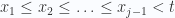
   To do a detailed analysis of the running time of this algorithm, you need to know how many times statement (**) is executed vs skipped. A related, perhaps simpler, question is this: assuming that the six numbers are all distinct and equally likely to be in any order (e.g., they might as well be a random permutation of 1, 2, …, 6), let the random variable X be the number of times the "if" test in (*) is false before the first time statement (**) is executed (if ever). I.e., X=2 means that the 0-th array element was larger than elements 1 and 2, but smaller than element 3.

   Find the probability mass function for X.

   Find E[X].

   Find Var[X].

2. Poisson approximation. The expected number of typos in on a page of The Hunger Games is 0.2. What is the probability that the next page you read contains (a) 0 errors? (b) 2 or more errors? Explain your reasoning.

3. Let N be an arbitrary random variable that takes only non-negative integer values. Prove that

   

Extra credit

You will show that the randomized min-cut algorithm can be made to run in time.

First, show that if you run the algorithm for only t steps, then the probability of contracting some edge of the minimum cut is .

Now consider the following algorithm: Run the basic algorithm to four times. Then recurse on each of these 4 copies. Use the recursion tree method (or some other method you know about) to argue why the running time for this will be

Finally, the probability of success is the probability that not all the recursions fail to find the min-cut. Argue that the probability of success is at least . Conclude that we need to run the algorithm only times to get a 90% probability of success.

Thus the total running time is .

Lecture 15: Tail bounds

Hear are the slides. Reading assignment: BT, Section 5.1.

Lecture 14: Joint distributions and randomized min cuts

Here are the slides.

And wikipedia does a great job discussing Karger’s randomized min cut algorithm.

Lecture 13: Randomized algorithms and Quicksort

Here are some great notes from Avrim Blum describing randomized algorithms and two analyses of quicksort, one of which we did in class.

Lecture 12: More random variables

Here are the slides.

Worksheet for Section 4

Here is the worksheet for Section 4.

Many people found these questions challenging.  Here are some hints walking you through the solutions.  If you solve a problem, please post your answer in the comments for others to see.

Hints/Comments:

(1) Most people seemed to figure this out.  The first important conceptual challenge is realizing that the probability is simply a function, as in .  Secondly, some people didn’t remember the chain rule for derivatives.

(2) The way I like to prove this is to start with the right-hand side, .  Then, expand both using the definition of the expected value.  The next crucial step is to apply the lemma I discussed in section, which is simply the marginal distribution for two variables.  Finally, some manipulation of sums using the distributive property of addition will lead you to .

(3) Many people had trouble with this.  To make it simpler, assume for some value in the range  of .  Then, also assume and  .  Now, use the definitions of cumulative probability and expected value to arrive at the answer.

(4) First, write down (from the definition) the expected value of the random variable .  Now, try to see how you can manipulate the terms in the sum to make it look like the desired equation.  Remember that the range of  is not necessarily the same as the range of .

Homework #5

Due, in class: February 15th

For this homework, you will need to turn in your solutions in two parts. This is for ease of grading by the TAs. Problems 1-4 and 5-7 should be turned in on different sheets of paper (there will be two different piles).

In solving the problem sets, you are allowed to collaborate with fellow students taking the class, but remember that you are required to write up the solutions by yourself or with a single partner. If you do collaborate in any way, you must acknowledge, for each problem, the people you worked with on that problem.

The problems have been carefully chosen for their pedagogical value, and hence might be similar to those given in past offerings of this course at UW, or similar to other courses at other schools.  Using any pre-existing solutions from these sources, for from the web, constitutes a violation of the academic integrity you are expected to exemplify, and is strictly prohibited.

Most of the problems only require one or two key ideas for their solution.  It will help you a lot to spell out these main ideas so that you can get most of the credit for a problem even if you err on the finer details.

A final piece of advice:  Start working on the problem sets early!  Don’t wait until the day (or few days) before they’re due.

Problems

Part one

1. [Probability mass functions]

   Let X be a random variable that takes values {1,2,3,4,5,6,7,8,9,10} each with probability 1/10.

   Find the PMF of the random variable Y = X mod 4.

   Find the PMF of the random variable Y = 5 mod (X+1).

2. [Binomial PMF]

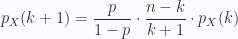
   Let X be a binomial random variable with distribution Bin(n,p). Write for its probability mass function (PMF). What is the value of ?

   Prove that for every k=0, 1, 2, …, the following recursive formula computes the PMF correctly.

   

3. [Facebook IPO]

   Since Facebook is about to be worth 100,000,000,000 dollars (yes, that’s the right number of zeros), Mark Zuckerberg chooses 6 interns and plays the following game. The interns are labeled 1,2,3,4,5,6. Then 6 distinct numbers are randomly distributed to the interns. Whenever two interns compare their numbers, the one with the highest number has to take a shot, and keep going. Initially, interns 1 and 2 compare their numbers; the “winner” then compares her number with that of intern 3, and so on. Let Y be the number of times intern 1 has to take a shot. What is the probability mass function of Y?

4. [The coin lottery]

   Suppose you toss independently a fair coin and you count the number of tosses until the first head appears.
   If this number is n, you receive dollars.
   What is the expected amount you will get?
   What’s the variance?
   How much would you pay to play this game?

Part two

1. [Mission impossible?]

   Tom Cruise and Katie Holmes claim they have ESP. To test their claim, we flip a fair coin 11 times and ask them to predict the outcome in advance. They get 8 out of 11 correct. Oprah throws a party and gives everyone a car. Now, what is the probability that they would have done at least this well without ESP?

2. [Advertising budgets]

   Extensive sampling has shown that when a person Google searches for “Gatorade” and a Vitamin Water ad appears, they click on it 15% of the time. Suppose that the Vitamin Water comes up with every “Gatorade” search and they are charged $1 whenever anyone clicks on their ad. Vitamin Water, unfortunately, has only $6000 to use for its daily advertising budget (come on, they sell water).

   Now, suppose you know that, since it’s Superbowl Sunday, there are going to be about 10,000 searches for Gatorade the next day. Prove to the Vitamin Water CEO that the probability of exceeding the advertising budget is at most 0.25.

   [Hint: First calculate E[X], where X = amount spent on advertising that day. Then show that if the probability of exceeding the budget is too big, then E[X] would be too big.]

3. [Guessing games]

   One of the 15 numbers 1, 2, …, 15 is chosen at random. You try to guess which number it is by only asking yes or no questions.
   You are charged $1 for each of the first ten questions you ask, and then $2 for each additional question.
   Let X be the amount of money you have to pay before determining the number. Compute E[X] for each of the two strategies:

   • Your ith question is “Is it i?” for i=1,2,3,4,5,6,7,8,9,10,11,12,13,14,15.
     

   • With each question, you try to eliminate one half of the remaining numbers, as nearly as possible.

Practice Midterm 2

The following practice midterm is in the same format as the in-class exam will be on Friday.

[Additional note: The real midterm will also have an extra credit problem for those who finish early.]

1. True/False
   
   • If B is an event with P(B)=0, then P(A|B) = 0 for any event A.

     False. If P(B)=0, then the conditional probability P(A|B) is undefined.

   • For random variables X and Y, E[X+Y]=E[X]+E[Y] if and only if X and Y are independent.

     False. E[X+Y]=E[X]+E[Y] holds for arbitrary random variables.

   • For any events A, B with P(A)>0 and P(B)>0, we have P(A|B)P(B) = P(B|A)P(A).

     True. Both are equal to P(AB) by the chain rule.

   • If X ~ Bin(5,1/3), then P(X=0)=(1/5)(1/3)=1/15.

     False. P(X=0)=(2/3)^5.

   • If a random variable X is always equal to 1, then Var[X]=0.

     True. In this case, E[X]=X=1, so Var[X]=E[(X-1)^2]=0.

2. Below is a picture of a network with 6 boosters. Suppose that each booster is active with probability . In order to a signal from A to arrive at B, at least two boosters on some A-B path must be active. What’s the probability that A can signal B?

   

   

   

3. Suppose that a certain stock goes up $1 with probability 2/3 and down $1 with probability 1/3 each day. The stock price starts at $3. What’s the expected price of the stock after 9 days?

   The expected change for one day is (2/3)(1) + (1/3)(-1) = 1/3. Thus by linearity of expectation, the expected change after 9 days is 9*(1/3)=3. So the expected price after 9 days is $6.

4. A dance class consists of 22 students, of which 10 are women and 12 are men. If 5 men and 5 women are to be chosen and then paired off, how many results are possible?

   

5. Suppose that for halloween, everyone gets a brown bag with two pieces of candy. Each piece is chosen randomly to be either chocolate or vanilla (so all possibilities CC, CV, VC, VV are equally likely). You reach into the bag and pull out one of the two candies at random. If you pull out a chocolate candy, what’s the probability that the other candy is vanilla?

   Using Bayes’ Rule:

   

   Now, use P(CV,VC)=1/2 and P(C|CV,VC)=1/2, and

   P(C)=P(C|CC) P(CC)+P(C|VV)P(VV) + P(C|CV)P(CV) + P(C|VC)P(VC) = 1/4 + 0 + 1/8 + 1/8 = 1/2.

   Thus P(CV,VC|C) = 1/2.

Practice Midterm 1

The following practice midterm is in the same format as the in-class exam will be on Friday.

1. True/False
   
   • Three events A, B, and C are independent if P(AB)=P(A)P(B), P(AC)=P(A)P(C) and P(BC)=P(B)P(C).

     False. To be independent, we would also need P(ABC)=P(A)P(B)P(C).

   • If a fair coin is flipped 5 times, the chance of getting exactly 3 heads is 10/32.

     True. The chances are .

   • If A and B are mutually exclusive events, then P(A or B) = P(A) + P(B).

     True.

   • If A and B are mutually exclusive events, then P(AB)=P(A)P(B).

     False. For mutually exclusive events, P(AB)=0.

   • If X ~ Bin(n,p) and Y ~ Poisson(pn) then X and Y have the same distribution.

     False. The Poisson approximation is not exact.

2. Below is a picture of a network with 6 routers. Suppose that each router fails independently with probability . What’s the probability that there is a route from A to B?

   

   

3. Suppose you roll a die 5 times, and X is the sum of the values. What is ?
   What is ? What is the variance of X?
   [Hint: For both calculations, use linearity of expectation!]

   Let be the 5 outcomes, so that . Linearity of expectation gives .

   Similarly, . Expanding out and using linearity of expectation yields . Hence,

4. How many ways are there to get a full house from a 5-card hand in a standard deck of 52 cards? (A full house means that the denominations on the cards are a,a,a,b,b for some a and b.)

   

5. Suppose that three cards are identical in form, except the first card has both sides colored red, the second card has both sides colored black, and the third card has one side colored red and the other colored black. The three cards are in mixed in a hat, and one card is selected randomly and put down on the ground. If the upper side of the chosen card is red, what is the probability the other side is black?

   Let RR, BB, RB denote the events that the chosen card is all red, all black, or red and black. Then,

   

   Computing these conditional probabilities yields